Predicting U.S. Soybean Yield with Climate Data
An end-to-end machine learning project on U.S. soybean yield prediction
Summary
This post walks through my end-to-end machine learning project on predicting U.S. soybean annual yield based on local climate conditions. We cover all key steps of a machine learning workflow, including ideation, feature selection, cross validation, baseline modeling, hyperparameter tuning, and model deployment. We employed annual soybean yield data and monthly climate variables during the historical period from 1981 to 2016. The model was trained on annual soybean yield data and monthly climate variables from 1981 to 2015, with 2016 used as the test set. We found that XGBRegressor performed the best among the regression algorithms (including linear and tree-based models) tested in this project. Our model achieved an \(R^2\) of ~0.9, demonstrating a strong ability to predict U.S. soybean annual yield based on climate conditions. Please refer to this repo for the project’s code.
Introduction
Soybean is a vital source of protein for both human and animal nutrition, but its yield is highly sensitive to weather and climate variability. High temperatures and low soil moisture, particularly during the summer reproductive period, can significantly reduce soybean yields (Hamed et al., 2021). Early-season excessive precipitation can also negatively impact soybean yields by restricting root development, causing nutrient leaching, and increasing disease susceptibility (Ortiz-Bobea et al., 2019).
This project is motivated by two questions:
- Can we build a machine learning model that predicts local annual soybean yield in the United States based on local climate conditions?
- Which climatic factors contribute most to the soybean yield prediction?
Figure 1 (source) illustrates the life cycle of a typical end-to-end machine learning project, which consists of four main components: data preparation, feature selection, model training, and deployment. We closely followed this framework throughout the project.
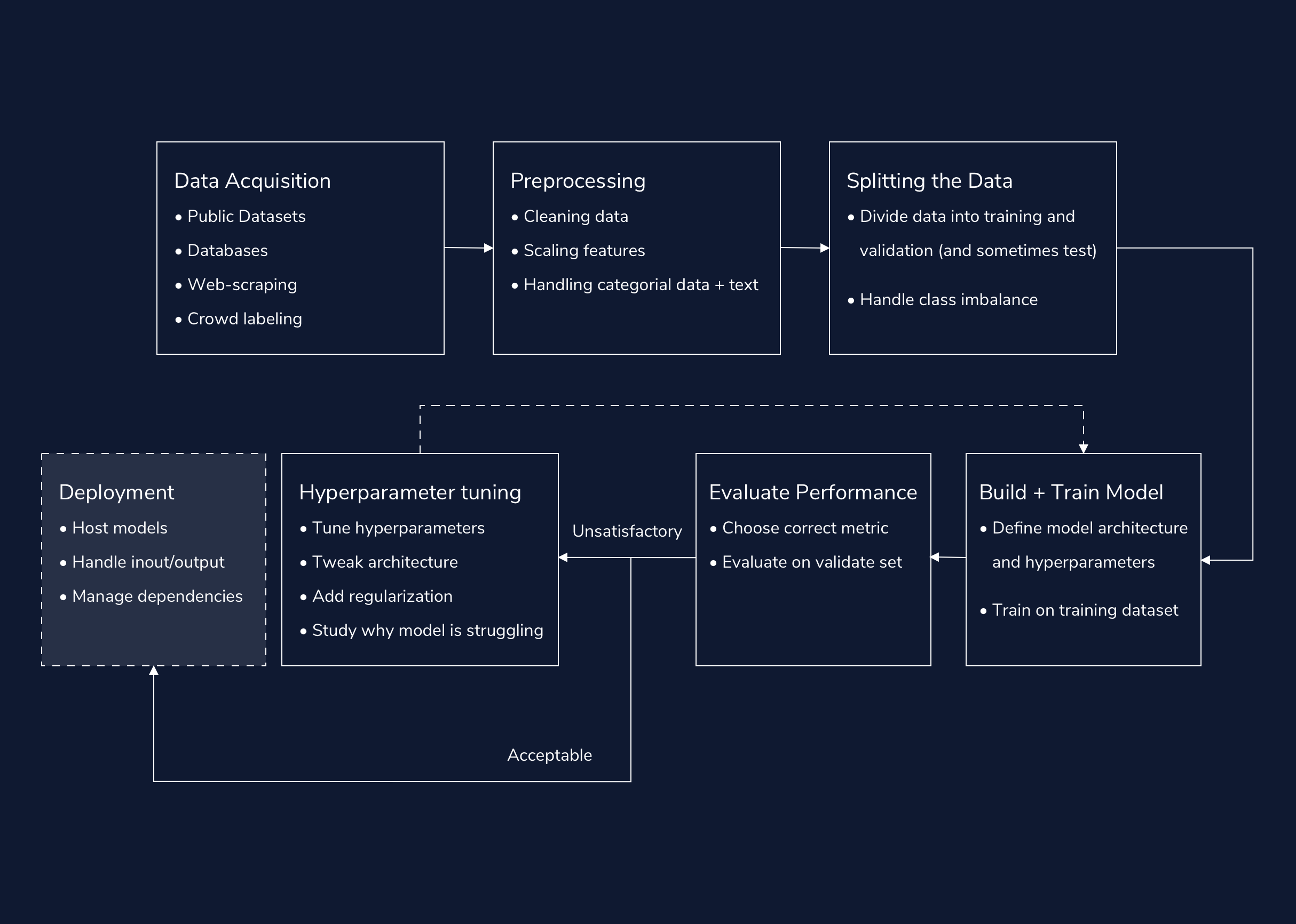
The reminder of the post is structured as follows. We first introduce the dataset and conduct an exploratory data analysis to examine the temporal and spatial patterns of the historical U.S. soybean yield. We then describe the feature selection process that constructed the training dataset. The model training section covers key aspects of model development. Finally, we discuss the deployment process and conclude with an overview of caveats and potential directions for future work.
Data
We focused on two datasets: one for soybean yield and the other for climate variables. Historical annual soybean yield was provided by the Global Dataset of Historical Yields (GDHY) (lizumi and Sakai, 2020), where crop yield is defined as production per unit harvested area (\(t\) \(ha^{-1}\)). For climate variables, we used monthly model outputs from the North American Land Data Assimilation System (NLDAS) (Mitchell et al. 2004). The NLDAS dataset provides near-surface climate variables, including surface energy fluxes, surface water flux and storage, soil moisture, temperature, and land surface parameters. Both GDHY and NLDAS are land-based datasets, meaning that values over the ocean appear as NaNs. We focus on the period 1981-2016, covering the spatial domain \(235.25^{\circ} - 292.75^{\circ}E, 25.25^{\circ} - 52.75^{\circ}N\), which encompasses the primary continental regions in the U.S.
Exploratory Data Analysis (EDA)
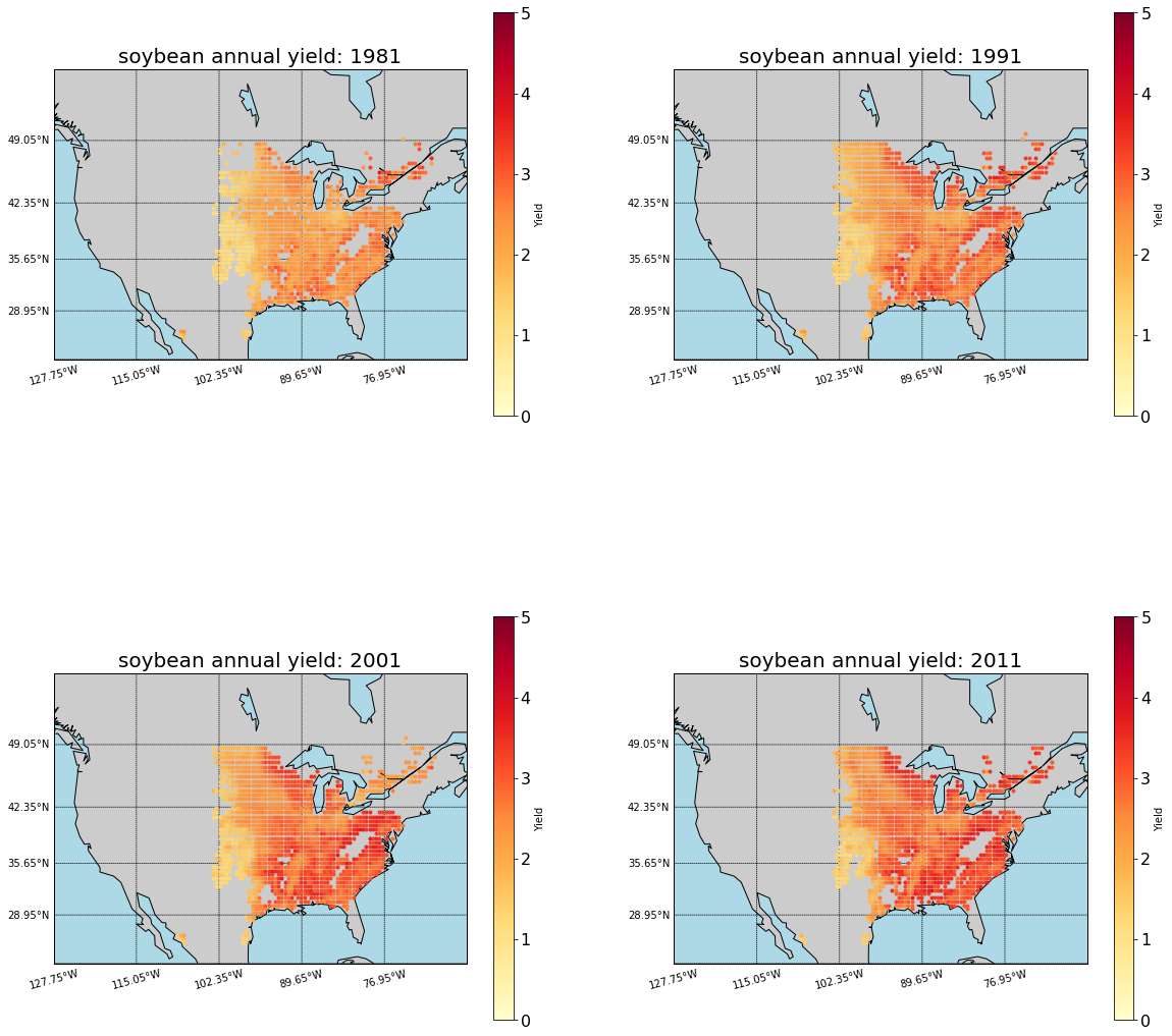
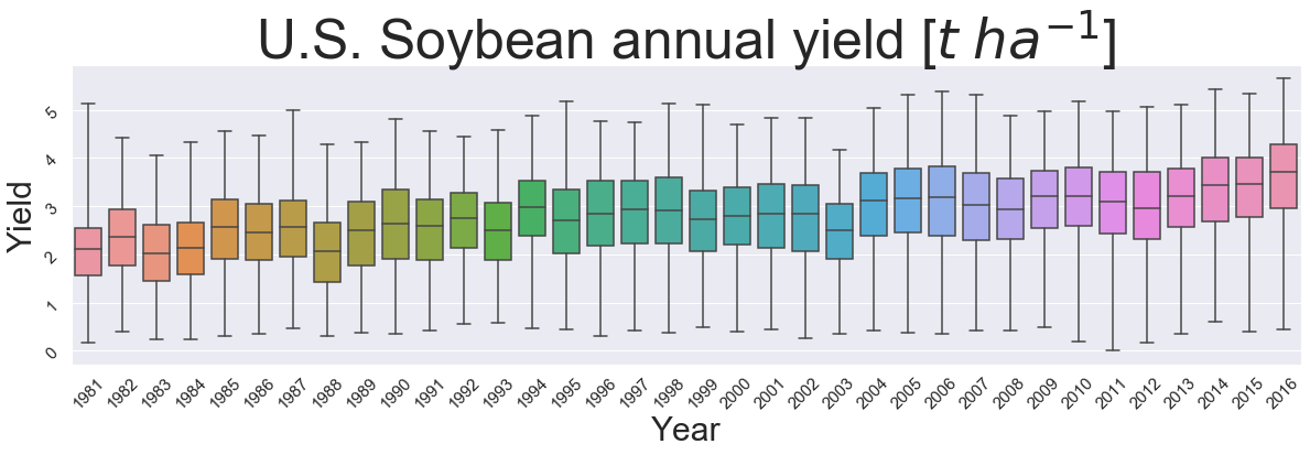
To better understand U.S. soybean production, we conducted an exploratory data analysis (Figures 2-5). The majority of soybean production is concentrated in the eastern and midwestern states, while the Great Plains region has relatively lower production density (Figure 2). To complement this spatial view, Figure 3 presents a boxplot of the interquartile range (IQR) across all soybean production grid points for each year, highlighting spatial variations in yield Both local soybean yield and its spatial spread exhibit year-to-year variability (Figures 2-3).
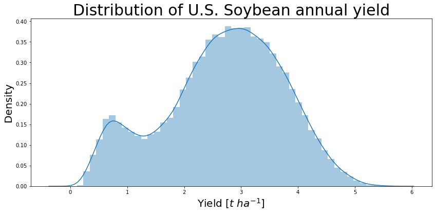
Statistical analysis reveals that U.S. soybean annual yield follows a bimodal distribution (Figure 4), suggesting that not all soybean-producing regions behave uniformly. We hypothesize that this bimodal pattern arises from differences between high-production areas (Midwestern and Eastern states) and lower-production areas (Great Plains) The left mode of the distribution likely corresponds to the Great Plains, while the right mode represents more densely cultivated regions.
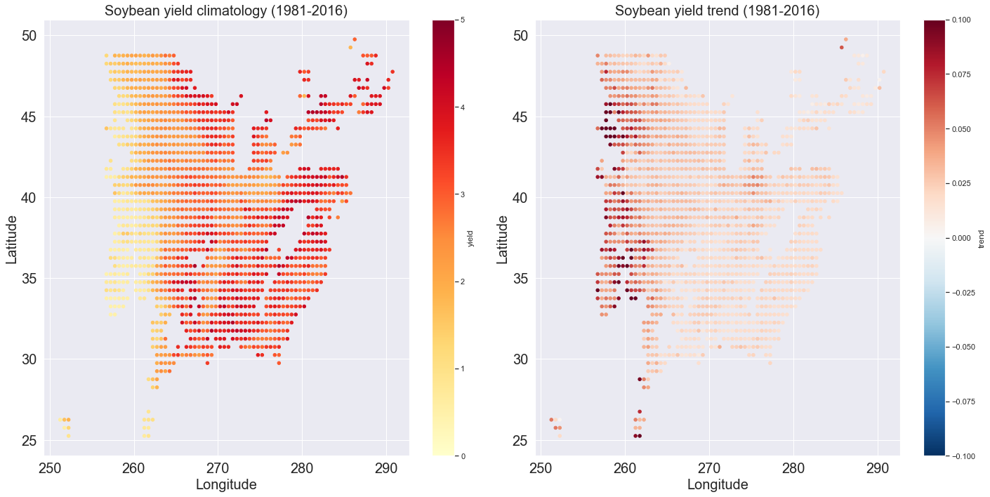
Both climatology and long-term trends display a west-east dipole pattern, further the Great Plains apart from other areas(Figure 5). Climatologically, soybean yield is lower in the Great Plains compared to other regions. The long-term trend, however, highlights the Great Plains as a hotspot area that experienced notable increase in soybean yield from 1981 to 2016. The overall increasing trend in the U.S. Soybean yield aligns with what we observed in Figure 3.
In this project, we train a unified model for all soybean production regions across the U.S. This approach assumes that the causal relationship between local climate conditions and soybean yield is consistent across all soybean production regions. We acknowledge that this is an oversimplification and we discuss its limitations in the Caveats and Future Work section.
We merged the GDHY and NLDAS datasets by matching the lat, lon, and year features (see Figure 6 for a screenshot of the merged dataset; see section 4.1 in this notebook). The resulting DataFrame contains over 600 climate features from NLDAS. We will perform feature selection in the next section.

Feature selection
Feature selection requires critical thinking and iterative analysis, making it the most tedious component of this project. Our goal is to narrow down the climate features to a subset that most likely affect soybean yield. This section outlines our thought process for feature selection. Detailed calculations and reasoning can be found in this notebook and this notebook.
Key considerations for feature selection:
- Feature selection should only be performed using the training dataset to prevent bias in feature and model choice from the test set.
- Feature selection does not always guarantee improved predictions.
- Linear and non-linear feature selection methods may yield conflicting results. When this happens, we rely on domain knowledge and our understanding of the problem to make decisions.
Feature selection process
We break the feature selection process into two phases:
- Phase 1: Initial feature filtering based on correlation analysis and domain knowledge.
- Phase 2: Further refinement using scikit-learn’s feature selection methods. We used features derived from Phase 1 to build baseline models, and used the refined features from Phase 2 for final model selection (see the
Model Developmentsection).
Phase 1: Initial Filtering
We followed these key principles in Phase 1:
- Temporal consideration:
- Most U.S. soybeans are planted in May and early June and harvested in late September and October (Source: USDA). Thus, we only consider climate features during months before October, removing November and December variables from the current year.
- Besides current-year climate, we explored whether past-year climate conditions matter. In particular, we explored past year’s annual total rainfall, past winter’s snowfall, rainfall, and soil moisture.
- Correlation analysis:
- We examined correlation between annual yield and climate features to identify important features. We kept variables with strong correlation with yield, and discarded the rest.
- Since some relationships between climate and yield are nonlinear, we kept certain features despite weak linear correlations if they were scientifically relevant.
- Redundant feature removal:
- We aggregated (e.g., seasonal averages) climate variables that are highly auto-correlated across months to avoid redundancy.
- Some climate variables exhibit strong cross-correlations, andi we only kept the most relevant ones.
- We excluded vegetation and land cover features (such as leaf area index) that directly reflect the yield data during the soybean growing and harvest season.
- Feature engineering: We created new features when necessary. For example, we derived an evaporative fraction using surface energy fluxes and used it instead of latent and sensible heat fluxes to simplify the feature set.
Phase 2: scikit-learn based feature selection methods
In Phase 2, we refined the feature set using various scikit-learn methods: VarianceThreshold, f_regression, mutual_info_regression, Lasso, and SelectFromModel. Although typically fewer methods are needed in practical applications, here we experimented with multiple approaches for the sake of practice. More details can be found in this notebook.
Model Development
Cross-validation
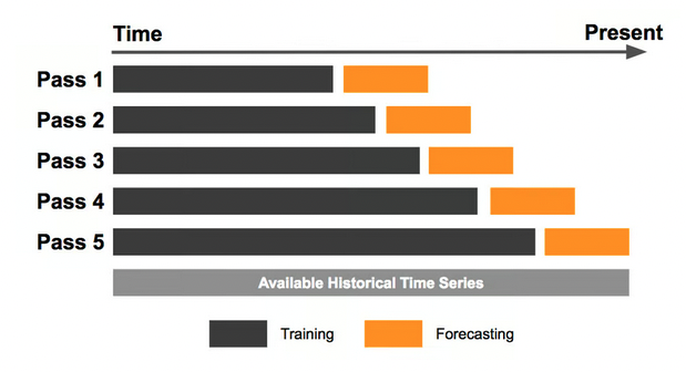
Cross-validation helps reduce overfitting in machine learning models. While scikit-learn’s train_test_split` method allows for random splitting of data, it is not suitable for our problem due to the sequential nature of the dataset. Instead, we implemented an expanding window backtesting procedure for cross-validation (Figure 7). Using this approach, we created a 5-fold split in the training set, ensuring that the test size remained constant across splits for comparability in their performance statistics:
- Split 1: train on 1980-2010, test on 2011
- Split 2: train on 1980-2011, test on 2012
- Split 3: train on 1980-2012, test on 2013
- Split 4: train on 1980-2013, test on 2014
- Split 5: train on 1980-2014, test on 2015
This method ensures that each model is trained on an expanding historical dataset, reflecting real-world forecasting conditions where future predictions are based only on past information.
Model selection
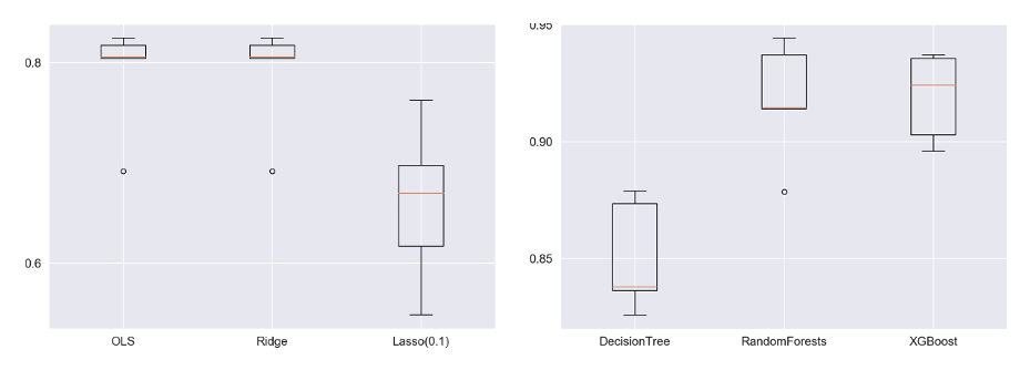
We first explored both linear models (OLS, Ridge, Lasso) and tree-based models (Decision Tree, Random Forest, XGBoost) to build baseline models. We used both \(R^2\) and RMSE to evaluate model performance. Not surprisingly, tree-based models outperformed linear models, with XGBoost achieving the best performance among the three tree-based models (Figure 8).
Hyperparameter tuning
We focused on tuning the following XGBoost hyperparameters to control overfitting:
-
n_estimators: Number of rounds for boosting. -
learning_rate: Step size shrinkage used in update to prevent overfitting. -
colsample_bytree: Subsample ratio of columns when constructing each tree -
subsample: Subsample ratio of the training instances. -
gamma: Minimum loss reduction required to split a leaf node of the tree; higher values make the algorithm more conservative. -
min_child_weight: Minimum sum of instance weights needed in a child; higher values make the algorithm more conservative. -max_depth: Maximum depth of a tree; higher values increase model complexity and risk of overfitting. -
reg_alpha: L1 regularization term on weights; higher values make the model more conservative.
Grid Search, Random Search, and Bayesian Optimization are commonly used hyperparameter tuning methods. We tested both Random Search and Bayesian Optimization (via Optuna). We selected the RandomizedSearchCV-tuned parameters as they produced a slightly higher \(R^2\) value.
Feature importance
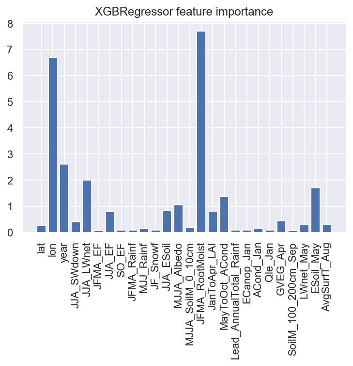
We used XGBoost’s built-in function to evaluate feature importance (Figure 9). Both longitude and year emerge as key features, reflecting the spatial-temporal nature of soybean yield prediction. Longitude serves as a proxy for geographic differences in soybean production, as observed in the EDA, while year likely captures long-term trends affecting yield. Several variables related to soil moisture content also stand out, including spring and summer soil moisture and summertime evaporative fraction. Springtime leaf area index also contributes to yield prediction, likely because it reflects pre-season vegetation health, which could correlate with soil fertility and growing conditions.
Inference and Deployment
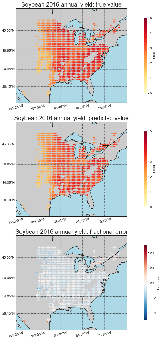
How well does the model perform in 2016 soybean annual yield? Figure 10 compares the true versus predicted values, suggesting that the model does a decent job in capturing both the spatial pattern and local magnitude of soybean yield. However, the model overall tends to underestimate annual yield c, while overestimating yield in some localized areas. We did not investigate the cause of this underestimation, which could be an area for future analysis. We deployed the trained XGBoost model on AWS EC2, and built a web interface using Flask, basic css and javascript.
Caveats and Future Work
In this section, we discuss several limitations of the current approach and potential future improvements.
Limited predictors
Unlike some other crops (e.g. corn) that are strongly influenced by soil type, drainage, population, row width, tillage and other physical and human factors, soybean yield is more dependent on the natural environment (Source: Stack the odds for soybeans this spring). Still, additional factors such as genotype, soil type, and seeding experiments could improve our model’s predictability.
In this project, we focused solely on the predictive power of local monthly climate due to the lack of suitable datasets for other predictors. This limitation may have constrained our model’s predictability. Even for the climate data, we relied on a single source (NLDAS). Future work could involve testing alternative datasets that provide both atmospheric and land-based variables to validate or refine our findings.
Coarse timescale of crop yield
The crop yields data used in this project only provide annual yields, thus we lack information on the timing of soybean planting and seasonal growth cycle at each location and year. Several studies (Colet et al., 2023; Vann and Stokes, 2024) suggest that planting timing affects yield. Future work incorporating sub-annual yield estimates or phenological data could help capture these temporal variations.
Localized climate perspective
This work takes a localized perspective of climate impacts.hat is, we only considered impacts of local climate on local yield. However, large-scale climate patterns can also affect U.S. soybean yield through teleconnections. For example, El Niño-Southern Oscillation (ENSO) events can impact U.S. growing conditions by synchronizing climate risks across major agricultural regions (Anderson et al., 2018). Including remote climate indices as features could improve our understanding of remote climate influences on soybean yield.
Spatial variation
As shown in the EDA, U.S. soybean yield varies across the Great Plains, Midwest, and Eastern states. We hypothesize that different sub-regions are governed by different climate factors. Even a common set of climate features is relevant across all regions, their importance may vary by location. Future work could explore training separate models for different sub-regions to improve predictions for local areas.
LSTM as an alternative model architecture
Long Short-Term Memory (LSTM) networks are well-suited for time-series forecasting tasks. Given the temporal nature of our soybean yield prediction problem, incorporating LSTM in future work could provide valuable insights. Several studies have demonstrated the effectiveness of LSTMs in crop yield prediction (Sun et al, 2019; Bhimavarapu et al., 2023). However, while LSTMs excel at capturing sequential dependencies, they require larger datasets and are more computationally intensive than tree-based models like XGBoost.
References
Journal Articles:
- Anderson, W., Seager, R., Baethgen, W., & Cane, M. (2018). Trans-Pacific ENSO teleconnections pose a correlated risk to agriculture. Agricultural and Forest Meteorology. https://doi.org/10.1016/j.agrformet.2018.07.023
- Bhimavarapu, U., Battineni, G., & Chintalapudi, N. (2023). Improved optimization algorithm in LSTM to predict crop yield. Computers, 12(1), 10. https://doi.org/10.3390/computers12010010
- Colet, F., Lindsey, A. J., & Lindsey, L. E. (2023). Soybean planting date and seeding rate effect on grain yield and profitability. Agronomy Journal. https://doi.org/10.1002/agj2.21434
- Hamed, M. K., Vogel, M. M., Patricola, C. M., & Seneviratne, S. I. (2021). Impacts of compound hot–dry extremes on US soybean yields. Earth System Dynamics, 12(4), 1371–1386. https://doi.org/10.5194/esd-12-1371-2021
- Iizumi, T., & Sakai, T. (2020). The global dataset of historical yields for major crops 1981–2016. Scientific Data, 7(1), 97. https://doi.org/10.1038/s41597-020-0433-7
- Mitchell, K. E., Lohmann, D., Houser, P. R., Wood, E. F., Schaake, J. C., Robock, A., … & Cosgrove, B. A. (2004). The multi-institution North American Land Data Assimilation System (NLDAS): Utilizing multiple GCIP products and partners in a continental distributed hydrological modeling system. Journal of Geophysical Research: Atmospheres, 109(D7), D07S90. https://doi.org/10.1029/2003JD003823
- Ortiz-Bobea, A., Wang, H., Carrillo, C. M., & Ault, T. R. (2019). Unpacking the climatic drivers of U.S. agricultural yields. Environmental Research Letters, 14(6), 064003. https://doi.org/10.1088/1748-9326/ab1e75
- Sun, J., Di, L., Sun, Z., Shen, Y., & Lai, Z. (2019). County-level soybean yield prediction using deep CNN-LSTM model. Sensors, 19(20), 4363. https://doi.org/10.3390/s19204363
Online Tutorials & Blog Posts:
- Vann, R., & Stokes, D. J. (2024, January). How does soybean planting date impact plant height and soybean yield? NC State Extension. https://soybeans.ces.ncsu.edu/2024/01/how-does-soybean-planting-date-impact-plant-height-and-soybean-yield/
- AgWeb. (2024, February). Stack the odds for soybeans this spring. https://www.agweb.com/news/crops/soybeans/stack-odds-soybeans-spring
- XGBoost. (n.d.). XGBoost hyperparameter tuning guide. XGBoost Documentation. https://xgboost.readthedocs.io/en/stable/tutorials/param_tuning.html
- XGBoost. (n.d.). XGBoost parameters. XGBoost Documentation. https://xgboost.readthedocs.io/en/stable/parameter.html
- Amazon Web Services. (n.d.). Tune an XGBoost model in Amazon SageMaker. AWS Documentation. https://docs.aws.amazon.com/sagemaker/latest/dg/xgboost-tuning.html
- Uber. (n.d.). Omphalos: Uber’s point of interest engine for better user experiences. Uber Blog. https://www.uber.com/blog/omphalos/
- Towards Data Science. (2020, April). Grid search vs. random search vs. Bayesian optimization. https://towardsdatascience.com/grid-search-vs-random-search-vs-bayesian-optimization-2e68f57c3c46
- Practical Data Science. (n.d.). How to tune an XGBRegressor model with Optuna. https://practicaldatascience.co.uk/machine-learning/how-to-tune-an-xgbregressor-model-with-optuna
GitHub Repository:
- Kong, W. (2022). U.S. soybean yield prediction [GitHub repository]. https://github.com/wenwenkong/data-science-portfolio/tree/main/US_soybean_yield