GenAI with LLMs (4) Parameter-efficient fine-tuning
This post covers parameter-efficient fine-tuning from the Generative AI With LLMs course offered by DeepLearning.AI.
Why Parameter efficient fine-tuning (PEFT)
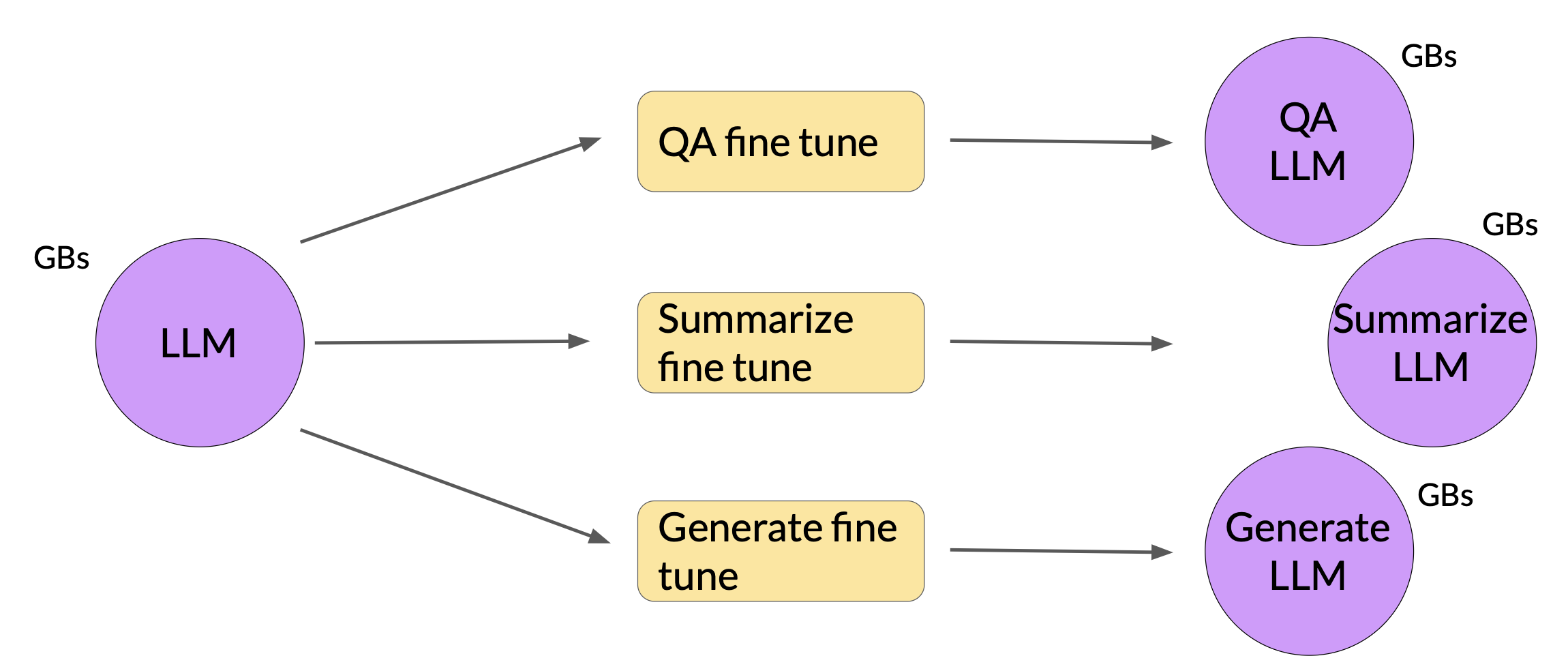
Full fine-tuning results in a new version of the original LLM for every task trained on. Each of the new version is the same size as the original model, so it can create an expensive storage problem if fine-funing for multiple tasks.
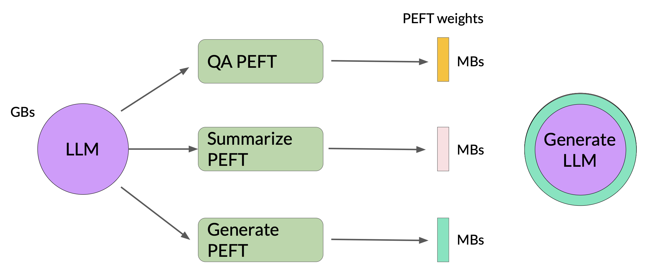
In contrast to full fine-tuning where every model weight is updated during supervised learning, PEFT only updates a small subset of parameters. Some PEFT techniques freeze most of the model weights and focus on fine-tuning a subset of existing model parameters, for example, particular layers or components. Other techniques don’t touch the model weights at all, and instead add a small number of new parameters or layers and fine-tune only the new components.
With PEFT, most if not all of the model weights are kept frozen. As a result, the number of trained parameters is much smaller than the number of parameters in the original LLM. In some cases, just 15-20 % of the original LLM weights. This makes the memory requirements for training much more manageable. In fact, PEFT can often be performed on a single GPU. And because the original LLM is only slightly modified or left unchanged, PEFT is less prone to the catastrophic forgetting problem of full fine-tuning.

PEFT methods
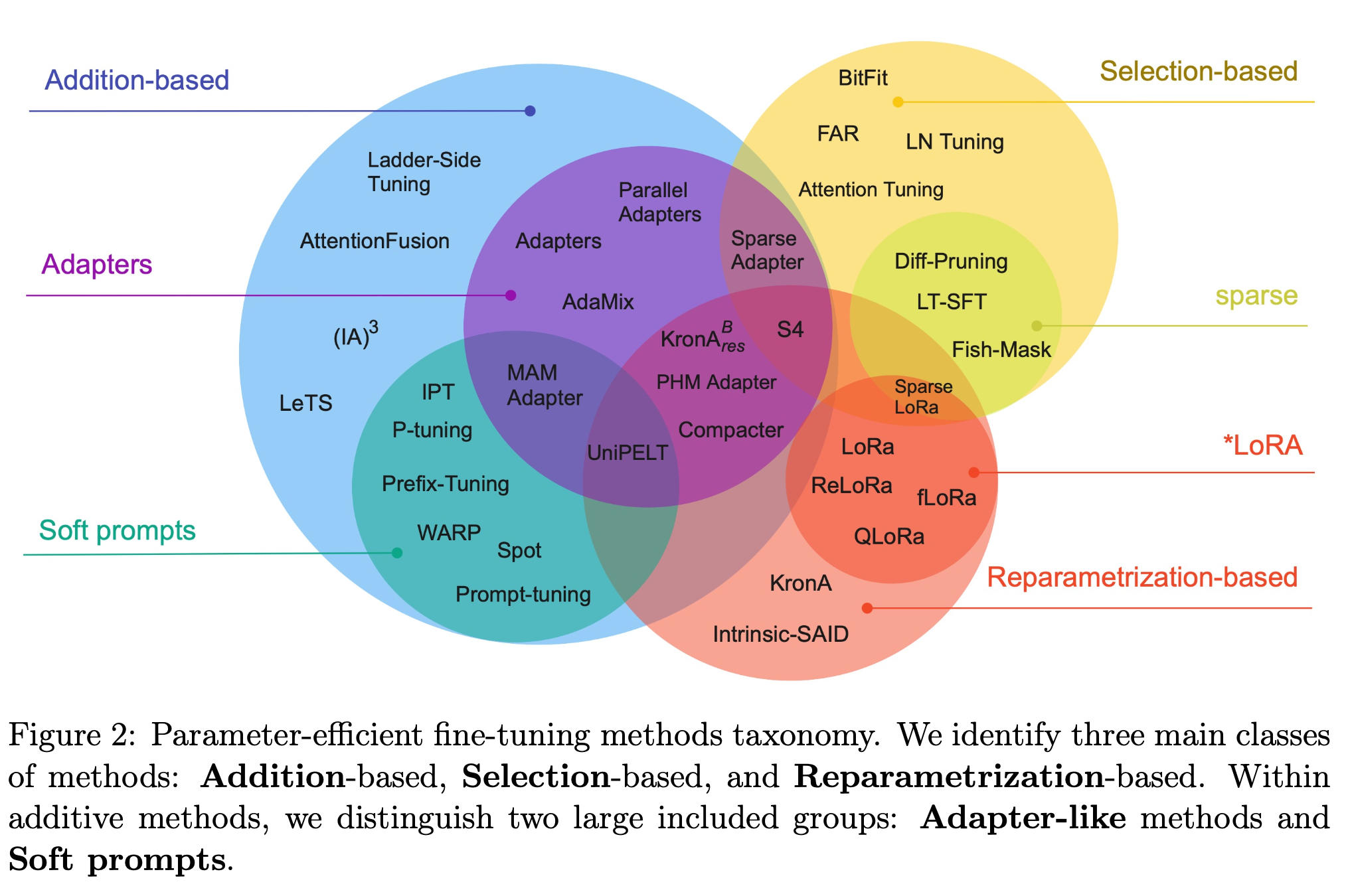
Selective
Select subset of initial LLM parameters to fine-tune. There are several methods you can take to identify which parameters you want to update. But performance of these methods (i.e., train only certain components, layers, or just individual parameter types) are mixed and there are significant trade-offs between parameter efficiency and compute efficiency.
Reparameterization
Reparameterize model weights using a low-rank representation. It works with the original LLM parameters, but reduces the number of parameters to train by creating new low rank transformations of the original network weights.
Additive
Add trainable layers or parameters to model. This fine-tuning method keeps all of the original LLM weights frozen and introducing new trainable components. For example,
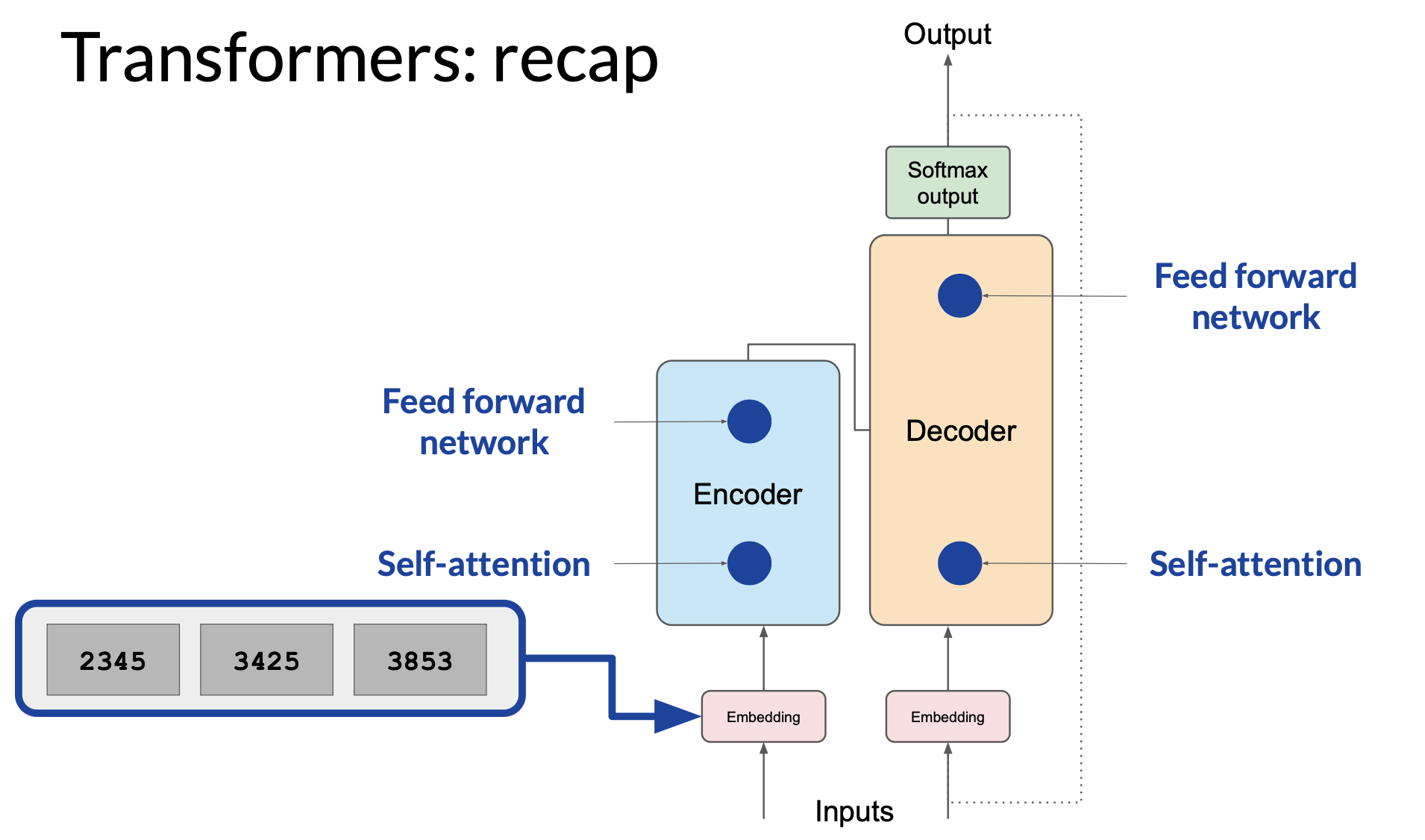
- Adapter adds new trainable layers to the architecture of the model, typically inside the encoder or decoder components after the attention or feed-forward layers.
- Soft prompts keep the model architecture fixed and frozen, and focus on manipulating the input to achieve better performance. This can be done by adding trainable parameters to the prompt embeddings or keeping the input fixed and retraining the embedding weights.
LoRA
LoRA == Low-Rank Adaptation of Large Language Models

LoRA workflow
-
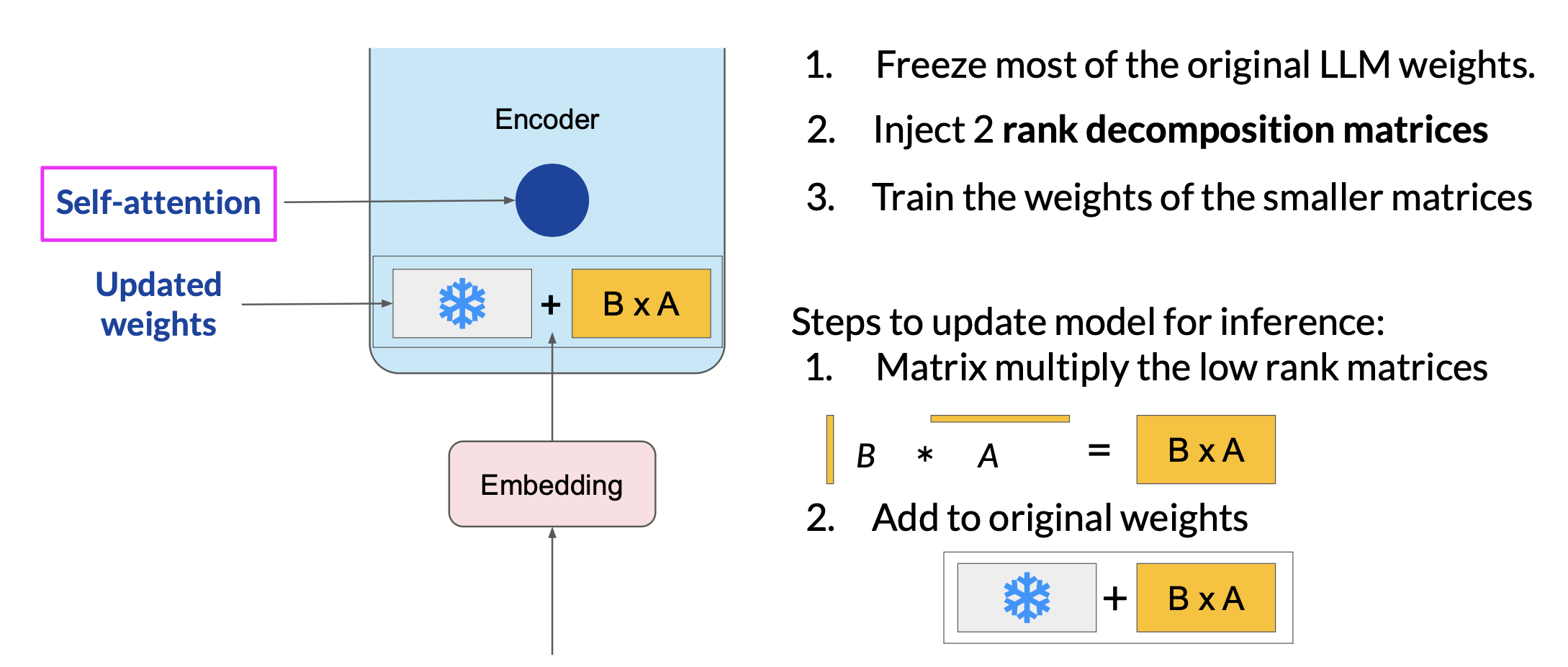
Freeze most of the original LLM weights, i.e. weights applied to embedding vectors
-
Inject 2 rank decomposition matrices
- The dimensions of the smaller matrices are set so their product is a matrix with the same dimensions as the weights they are modifying.
-
Train the weights of the smaller matrices
- Keep the original weights of the LLM frozen and train the smaller matrices.
-
Inference
- For inference, the two low-rank matrices are multiplied together to create a matrix with the same dimensions as the frozen weights. Add this to the original weights and replace them in the model with the updated values.
Note:
- Because the LoRA fine-tuned model has the same number of parameters with the original model, there is little to no impact on inferenc latency.
- Researchers have found that applying LoRA to just the self-attention layers of the model is often enough to fine-tune for a task and achieve performance gains. In principle, you can also use LoRA on other components like the feed-forward layers. However, since most of the parameters of LLMs are in the attention layers, you get the biggest savings in trainable parameters by applying LoRA to these weights matrices.
- Because LoRA allows you to significantly reduce the number of trainable parameters, you can often perform this PEFT method with a single GPU and avoid the need for a distributed cluster of GPUs.
LoRA: math behind
Use the base Transformer model presented by Vaswani et al. 2017 as an example, consider LoRA wight rank \(r = 8\).
Base weight:
\[W_0 \in \mathbb{R}^{d \times k} = \mathbb{R}^{512 \times 64} \Rightarrow 32{,}768 \text{ parameters}\]LoRA low-rank matrices:
\[A \in \mathbb{R}^{r \times k} = \mathbb{R}^{8 \times 64} \Rightarrow 512 \text{ parameters}\] \[B \in \mathbb{R}^{d \times r} = \mathbb{R}^{512 \times 8} \Rightarrow 4{,}096 \text{ parameters}\]Total LoRA parameters trained:
\[512 + 4096 = 4,608\]Parameter reduction:
\[1 - \frac{4608}{32768} = 0.859 \Rightarrow \text{~86% reduction}\]Understanding why the total parameters during the inference stays the same.
During training:
- The original weight matrix \(W_0\) is frozen
- Two small matrices \(A \in \mathbb{R}^{r \times k}\), \(B \in \mathbb{R}^{d \times r}\) are trained
- The effective weight becomes \(W = W_0 + \Delta W = W_0 + B \cdot A\)
- The model learns the low-rank update \(\Delta W\), which is far smaller in size then \(W_0\)
At inference:
- Merge the update \(B \cdot A\) into \(W_0\) ahead of time
- So still using a matrix of size \(d x k\), not adding more layers or extra computations during forward pass
- Thus, inference speed and memory stay the same as the original model
LoRA for different tasks
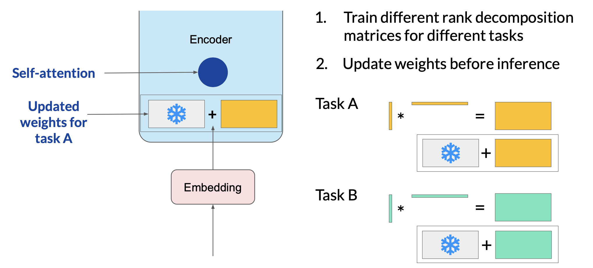
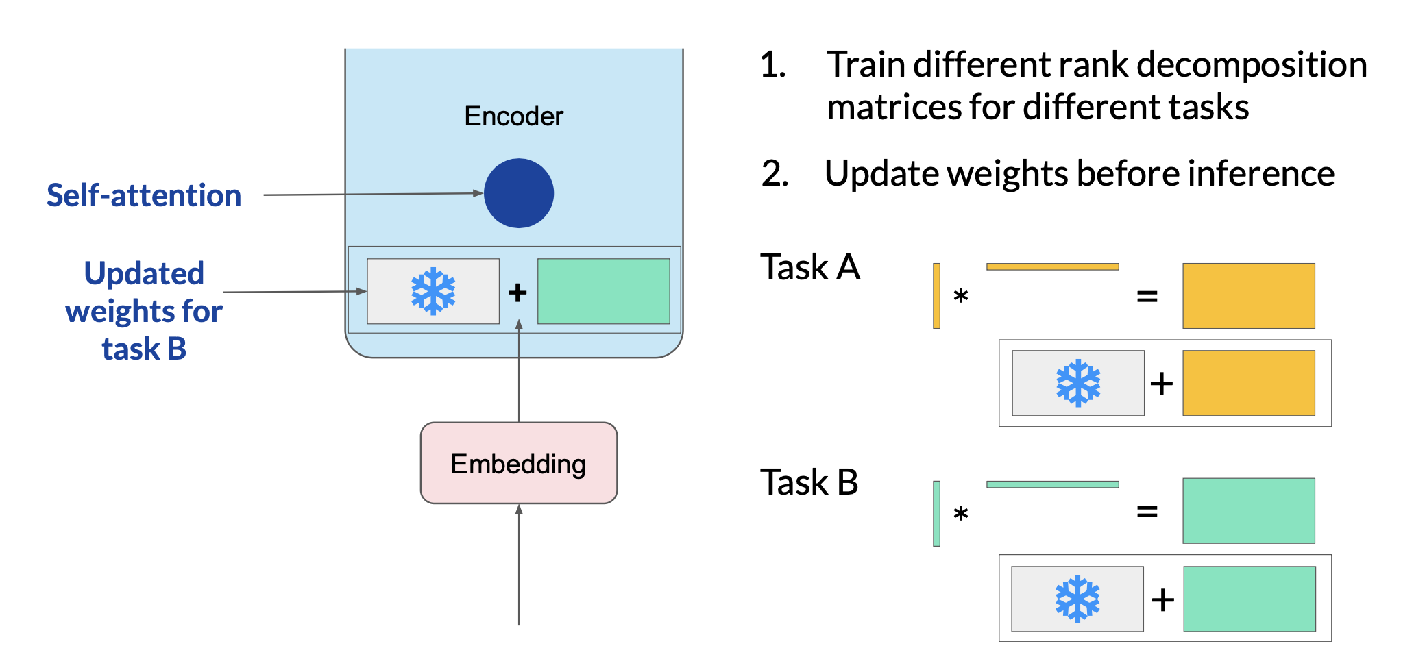
Since the rank-decomposition matrices are small, you can fine-tune a different set for each task and then switch them out at inference time by updating the weights.
Suppose you train a pair of LoRA matrices for a specific task, Task A. To carry out inference on this task, you would multiply these matrices together and then add the resulting matrix to the original frozen weights. You then take this summed weight matrix and replace the original weights where they appear in your model. You can then use this model to carry out inference on Task A. And you can repeat the same process for task B.
LoRA: other notes
ROUGE metrics from LoRA fine-tuning only slightly suffers compared to that from full fine-tuning.

How to choose the rank?
- The smaller the rank, the smaller number of trainable parameters, and the bigger saving on compute.
- Ranks in the range of 4 to 32 can provide a good trade-off between reducing trainable parameters and preserving performance.
- Optimizing the choice of rank is an ongoing area of research and best practices may evolve.

Soft prompt
Prompt tuning is not prompt engineering. With prompt tuning, you add additional trainable tokens to your prompt and leave it up to the supervised learning process to determine their optimal values. The set of trainable tokens is called a soft prompt, and it gets prepended to embedding vectors that represent your input text. The soft prompt vectors have the same length as the embedding vectors of the language tokens. Usually 20-100 tokens can be sufficient for good performance.
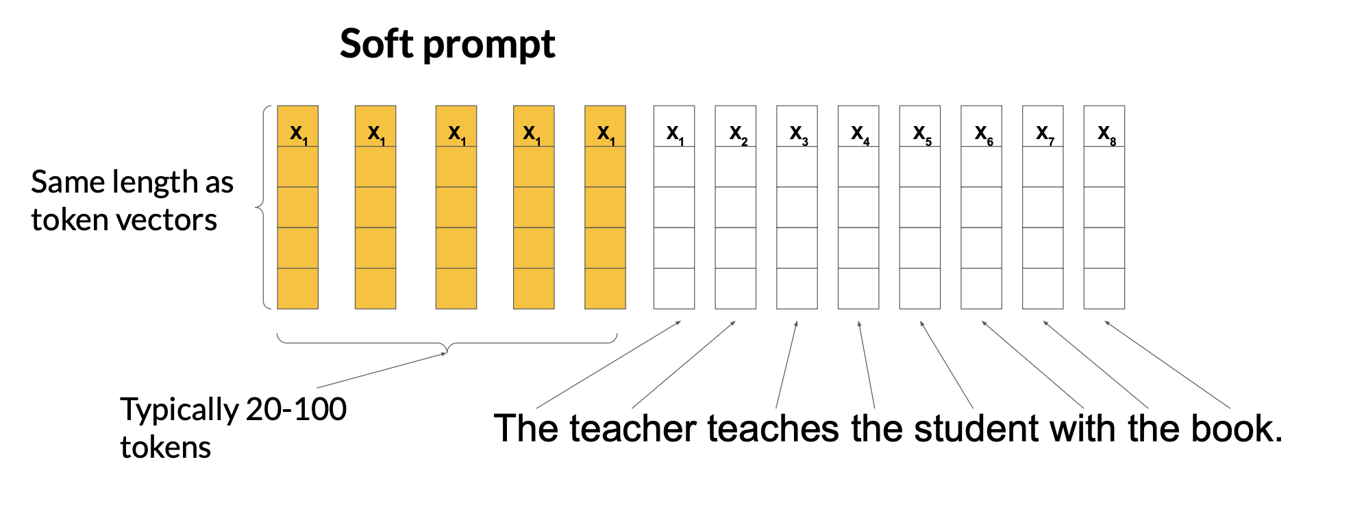
The tokens that represent natural language are hard in the sense that they each correspond to a fixed location in the embedding vector space. However, the soft prompts are not fixed discrete words of natural language. Instead, you can think of them as virtual tokens that can take on any value within the continuous multidimensional embedding space. Through supervised learning, the model learns the values for these virtual tokens that maximize performance for a given task.
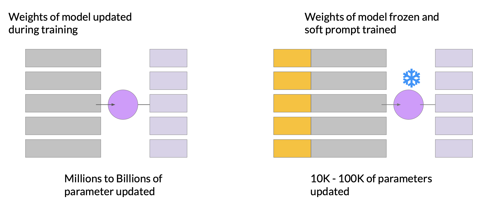
In full fine-tuning, the training data set consists of input prompts and output completions or labels. The weights of the LLM are updated during supervised learning. In contrast, with prompt tuning, the weights of the LLM are frozen and the underlying model does not get updated. Instead, the embedding vectors of the soft prompt gets updated over time optimize the model’s completion of the prompt. Prompt tuning is a very parameter efficient strategy because only a few parameters are being trained. Similar to LoRA, you can train a different set of soft prompts for each task and then easily swap them out at inference time.
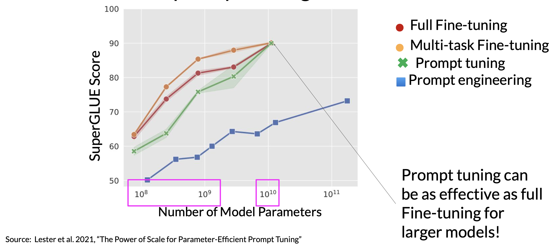
Prompt tuning doesn’t perform as well as full fine-tuning for smaller LLMs. However, as the model size increases, so does the performance of prompt tuning.
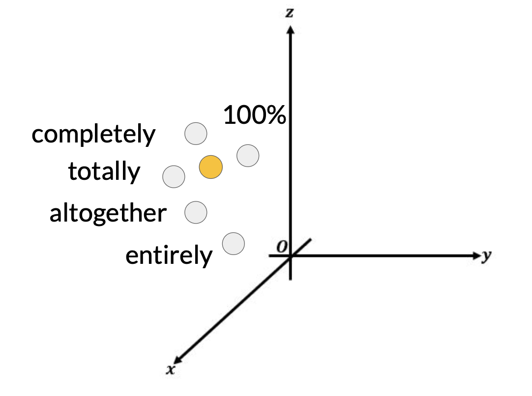
Because the soft prompt tokens can take any value within the continuous embedding vector space, the trained tokens don’t correspond to any known token, word, or phrase in the vocabulary of the LLM. Therefore interpretability of the virtual tokens can be a potential issue. An analysis of the nearest neighbor tokens to the soft prompt location shows that they form tight semantic clusters. That is, the words closest to the soft prompt tokens have similar meanings. The words identified usually have some meaning related to the task, suggesting that the prompts are learning word-like representations.
References
- Scaling Down to Scale Up: A Guide to Parameter-Efficient Fine-Tuning
- This paper provides a systematic overview of Parameter-Efficient Fine-tuning (PEFT) Methods in all three categories discussed in the lecture videos.
- On the Effectiveness of Parameter-Efficient Fine-Tuning
- The paper analyzes sparse fine-tuning methods for pre-trained models in NLP.
- LoRA Low-Rank Adaptation of Large Language Models
- This paper proposes a parameter-efficient fine-tuning method that makes use of low-rank decomposition matrices to reduce the number of trainable parameters needed for fine-tuning language models.
- QLoRA: Efficient Finetuning of Quantized LLMs
- This paper introduces an efficient method for fine-tuning large language models on a single GPU, based on quantization, achieving impressive results on benchmark tests.
- The Power of Scale for Parameter-Efficient Prompt Tuning
- The paper explores “prompt tuning,” a method for conditioning language models with learned soft prompts, achieving competitive performance compared to full fine-tuning and enabling model reuse for many tasks.