GenAI with LLMs (2) Pre-training
This post covers LLM pre-training and scaling laws from the Generative AI With LLMs course offered by DeepLearning.AI.
Model cards
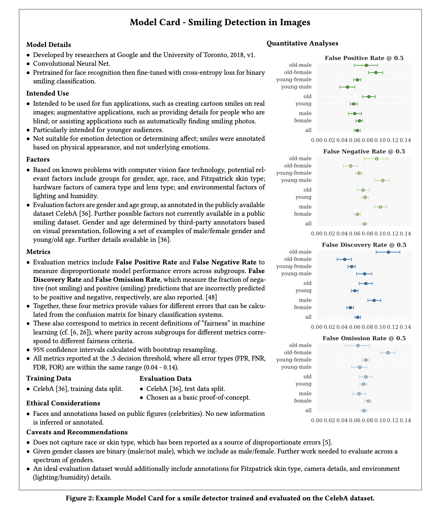
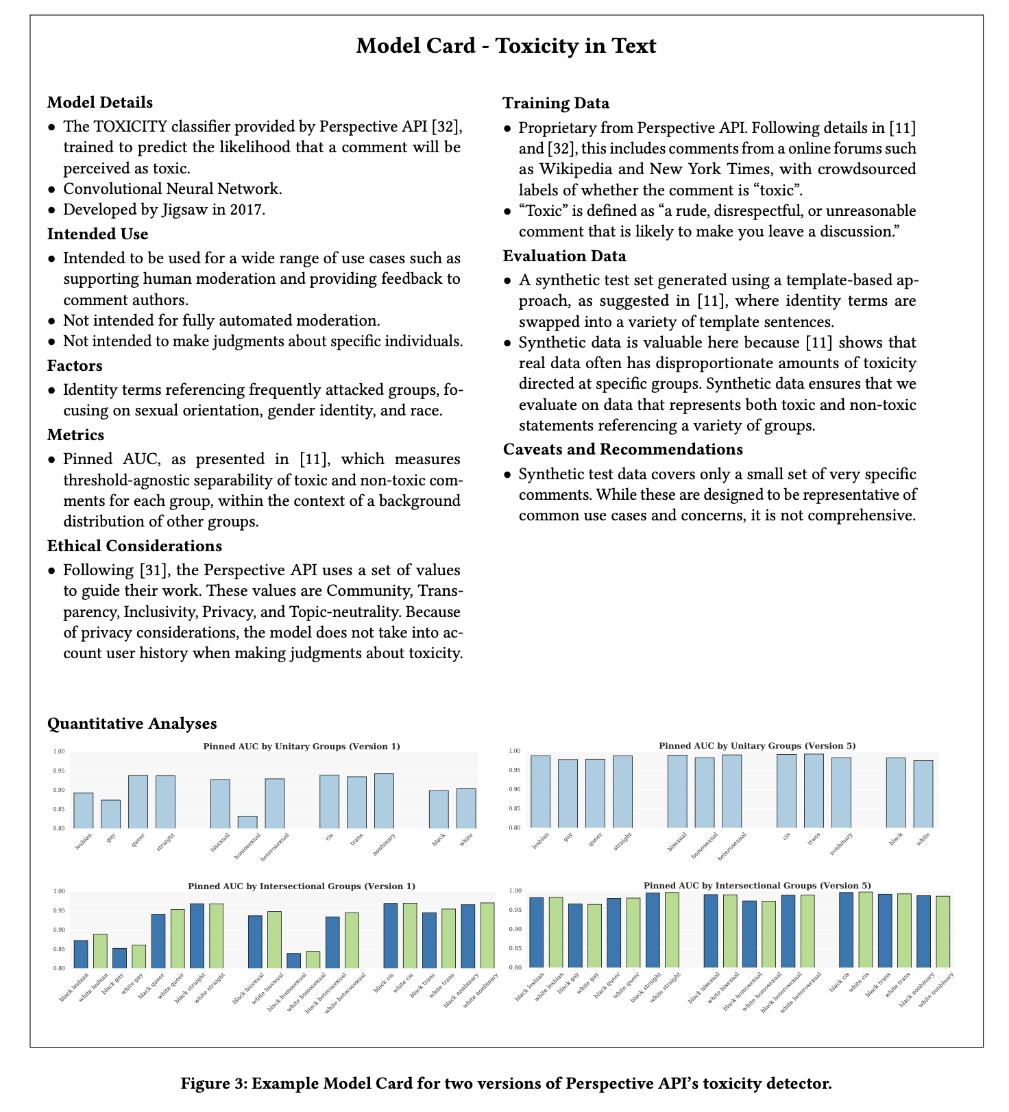
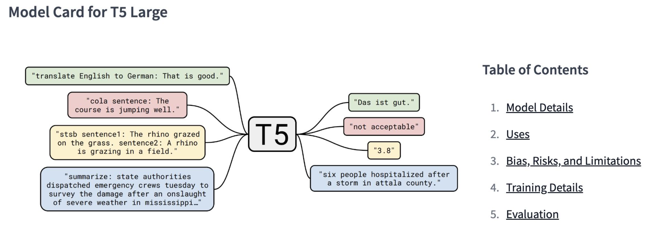
Model cards are useful for understanding how a model is trained, its use case, and known limitations. See here for a more complete definition from HuggingFace.
Figures 1-2 are two example model cards from Mitchel et al. (2018). Figure 3 is the model card for T5 Large, captured from the lecture slides.
Token filtering
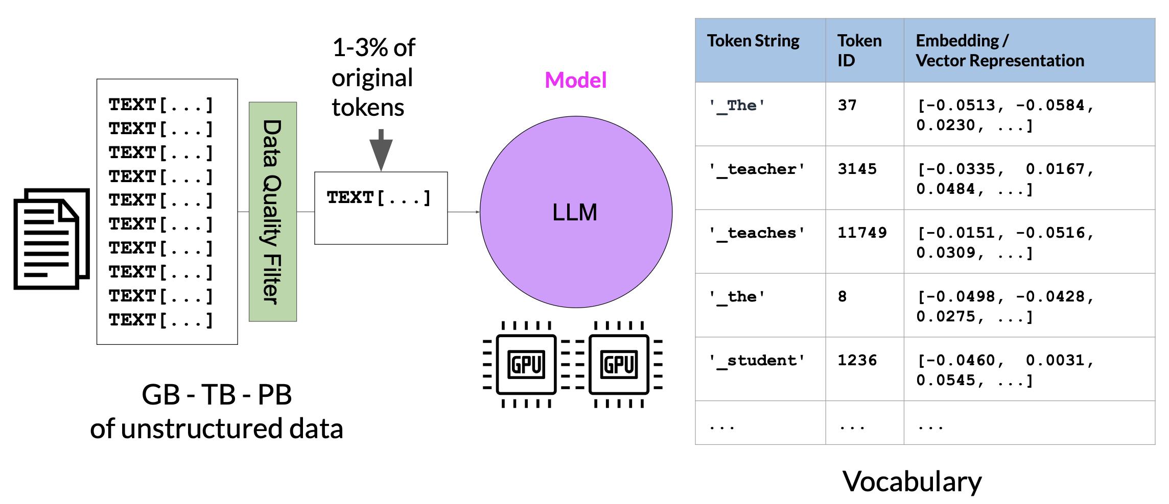
Only 1-3% of original tokens are used to train the LLM. We should consider this when we estimate how much data we need to collect if we decide to pre-train our own model. In other words, data quality control or bias removal is always needed to increase data quality before training. This refers to the token filtering or rejection process during LLM pre-training.
LLM developers all start from massive web-scale corpora, then spend huge effort on filtering, deduplicating, scoring for quality, and weighting data by domain or value. See GPT-4 Technical Report, LLaMA, and Chinchilla for details.
LLMs pre-training
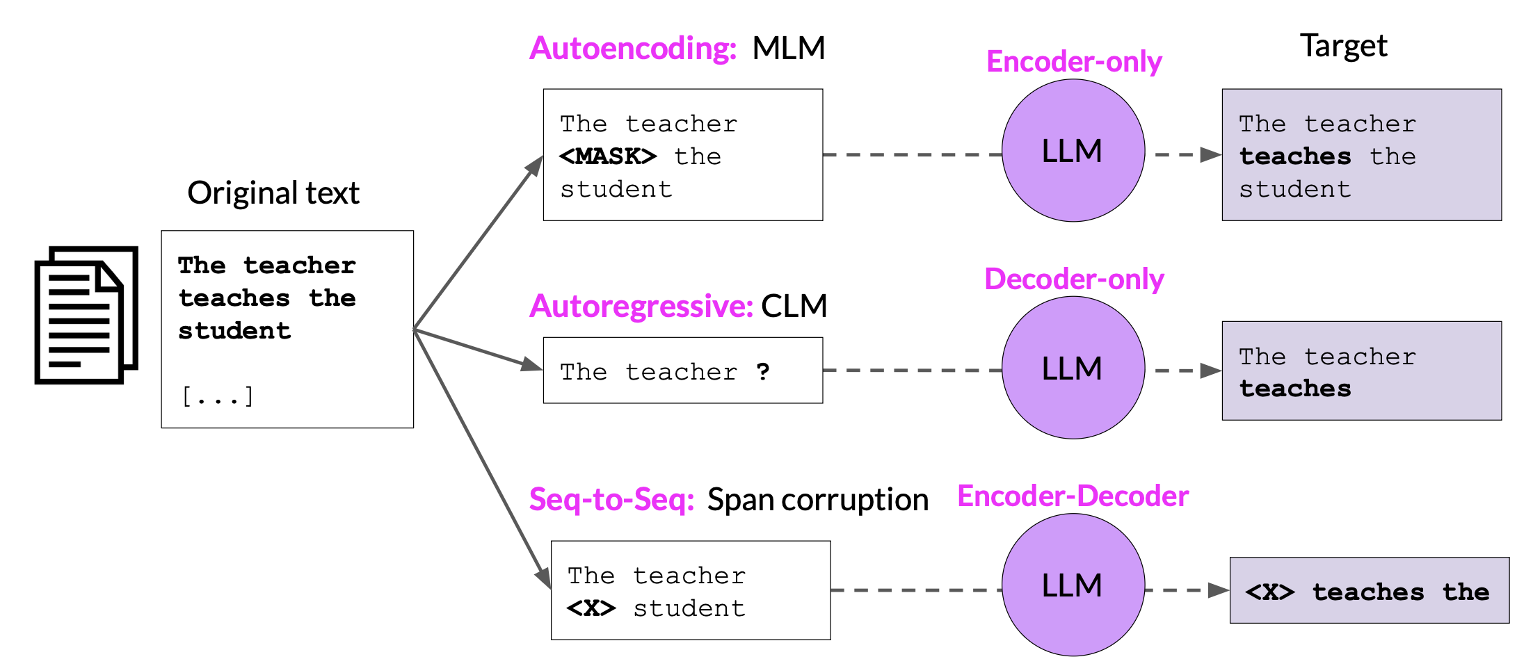
Different LLMs pretrain using different objectives - from denoising (such as BERT), to predicting next tokens (such as GPT), to reconstructing corrupted input using a sequence-to-sequence setup (such as T5 and BART). These design choices affect how models behave. For example, BERT is optimized for understanding tasks, GPT excels at generating fluent and coherent outputs. T5 and BART aim to balance both.
Autoencoding models
Autoencoding models like BERT are pre-trained using masked language modeling. In the context of autoencoding models, the pre-training task is often described as a “denoising” objective because the model learns to reconstruct the original text from a corrupted (noisy) version of it.
This setup provides the model with bi-directional context, meaning it can consider both preceding and following words when predicting masked tokens.
Autoregressive models
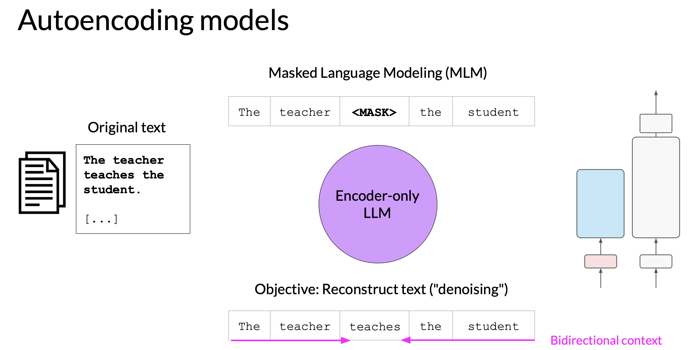
Autoregressive models are pretrained using causal language modeling, where the model learns to predict the next token based solely on the preceding sequence of tokens. Note: predicting the next token is sometimes called full language modeling by researchers.
This setup provides unidirectional context, meaning the model has no access to future tokens during training. Autoregressive models mask the input sequence and can only see the input tokens leading up to the token in question. The model has no knowledge of the end of the sequence. The model then iterates over the input sequence one by one to predict the following token.
Large decoder-only models, such as GPT, demonstrate strong ability in zero-shot and few-shot inferences, and can generalize well across a wide range of language tasks.
Seq2Seq models
Exact detail of pre-training varies from model to model.
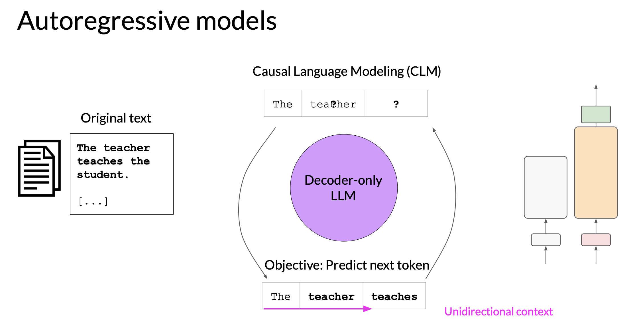
- A popular Seq2Seq model T5 pretrains the encoder using span corruption, which masks random sequences of input tokens. Those masked sequences are then replaced with a unique sentinel token. Sentinel tokens are special tokens added to the vocabulary, but do not correspond to any actual word from the input text. The decoder is then tasked with reconstructing the masked token sequences auto-regressively. The output is the sentinel token followed by the predicted tokens.
- BART combines the ideas of masked language modeling and causal language modeling within a seq2seq (encoder-decoder) framework. It corrupts text with various noise functions (e.g., setence shuffling, token masking), then uses a decoder to reconstruct the original text.
Model size
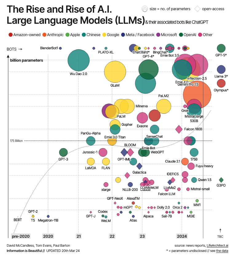
The growth of model size is powerd by
- introduction of transformer
- access to massive datasets
- more powerful compute resources
Compute challenge
CUDA, short for Compute Unified Device Architecture, is a collection of libraries and tools developed for NVIDIA GPUs to boost performance on common deep-learning operations, including matrix multiplication, among many others. Deep-learning libraries such as PyTorch and TensorFlow use CUDA extensively to handle the low-level, hardware-specific details, including data movement between CPU and GPU memory.

Quote from Generative AI on AWS: Building Context-Aware Multimodal Reasoning Applications (source):
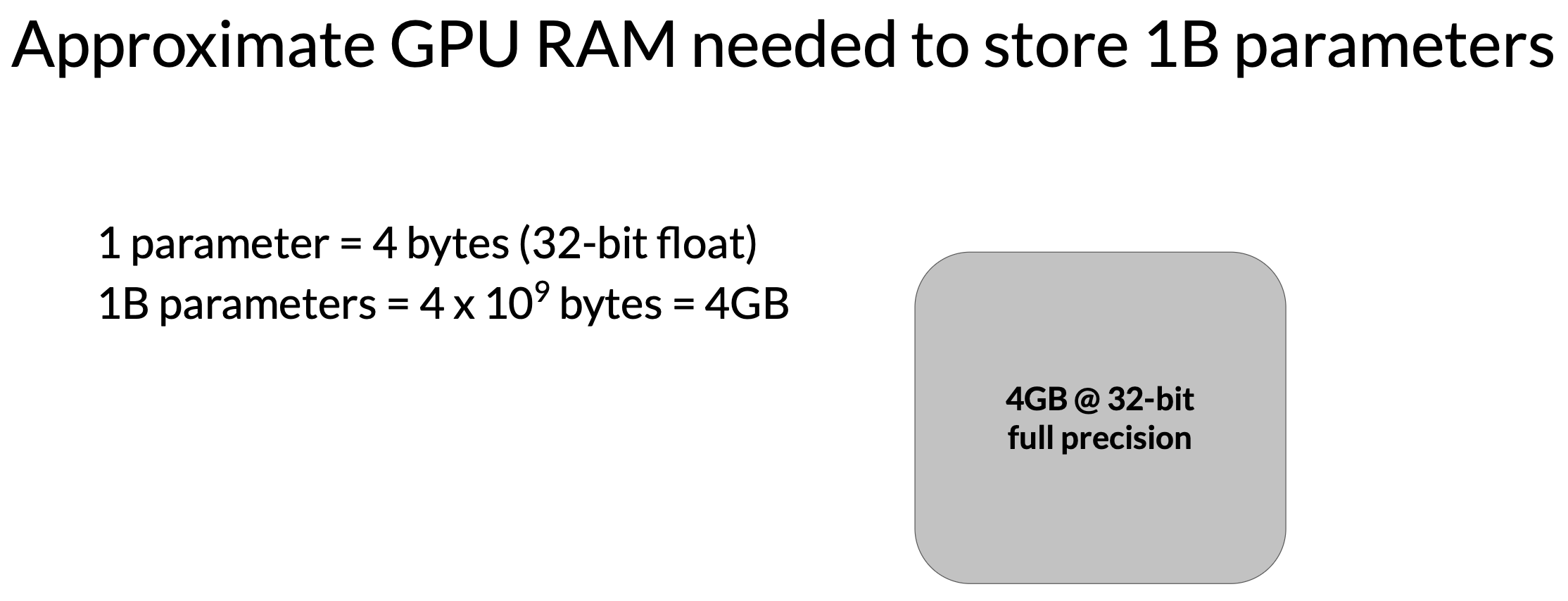
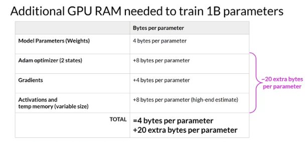
A single-model parameter, at full 32-bit precision, is represented by 4 bytes. Therefore, a 1-billion-parameter model requires 4GB of GPU RAM just to load the model into GPU RAM at full precision. If you want to also train the model, you need more GPU memory to store the states of the numerical optimizer, gradients, and activations, as well as any temporary variables used by your functions.
Quote from Generative AI on AWS: Building Context-Aware Multimodal Reasoning Applications (source):
When you experiment with training a model, it’s recommended that you start with batch_size=1 to find the memory boundaries of the model with just a single training example. You can then incrementally increase the batch size until you hit the CUDA out-of-memory error. This will determine the maximum batch size for the model and dataset. A larger batch size can often speed up your model training.
These additional components lead to approximately 12–20 extra bytes of GPU memory per model parameter. For example, to train a 1-billion-parameter model, you will need approximately 24 GB of GPU RAM at 32-bit full precision, six times the memory compared to just 4 GB of GPU RAM for loading the model

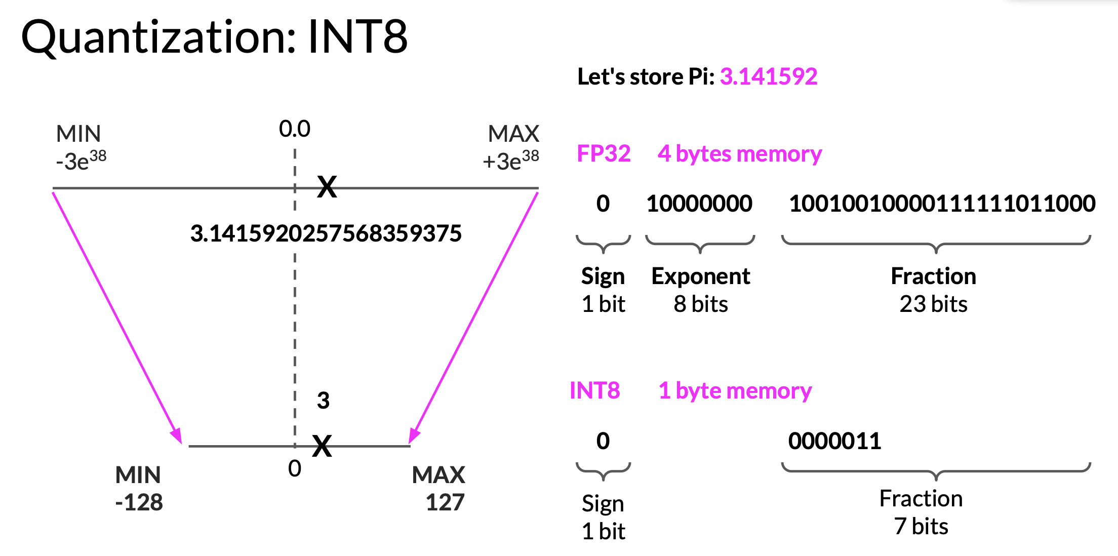
One technique we can use to reduce memory is called quantization. The idea is to reduce the memory required to store the model weights by reducing their precision from 32-bit floating point numbers to 16-bit (or 8-bit) floating point numbers. Quantization statistically projects the original 32-bit floating point numbers into a lower precision space, using scaling factors calculated based on the range of the original 32-bit floating point numbers.
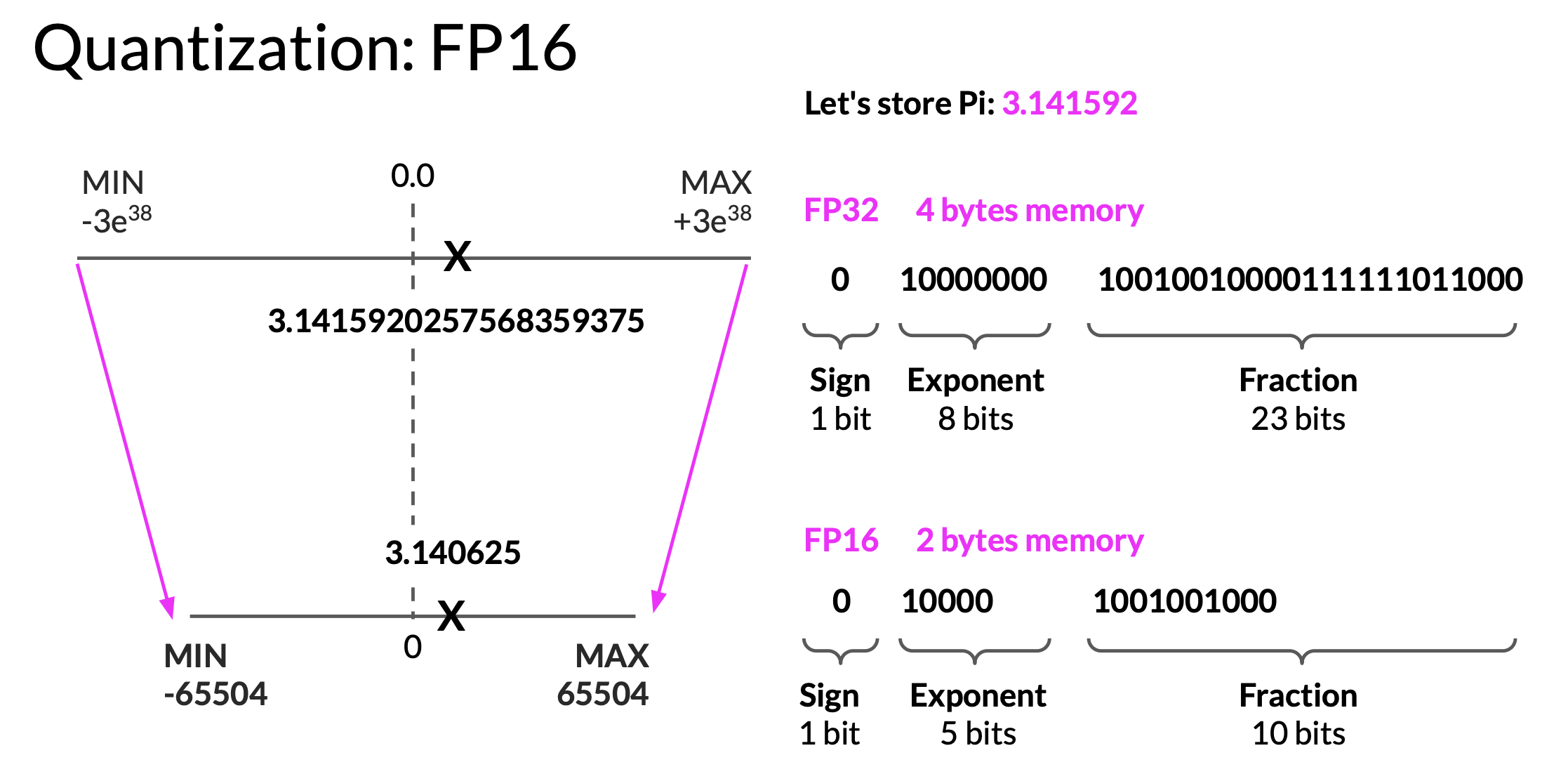
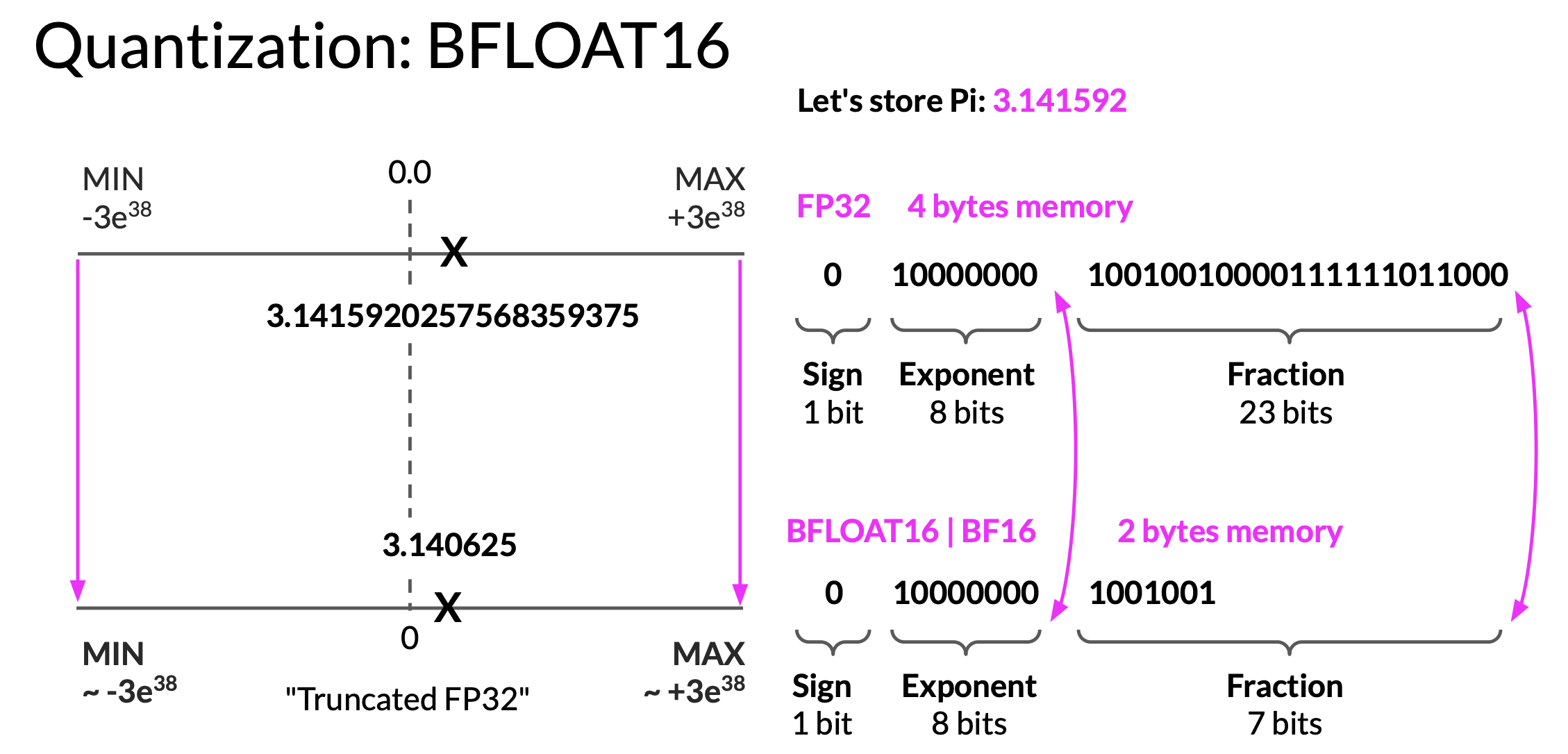
BFLOAT-16 (BF16, developed at Google Brain) has recently become a popular alternative to FP16.
- BF16 is a hybrid between half precision FP16 and full precision FP32.
- BF16 significantly helps with training stability and is supported by newer GPUs such as NVIDIA’s A100.
- BF16 is often described as truncated 32-bit float, as it captures the full dynamic range of the full 32-bit float that uses only 16-bits.
- BF16 uses the full 8 bits to represent the exponent, but truncates the fraction to just 7 bits.
- Downside: BF16 is not well suited for integer calculations, but these are relatively rare in deep learning.
Scalling law
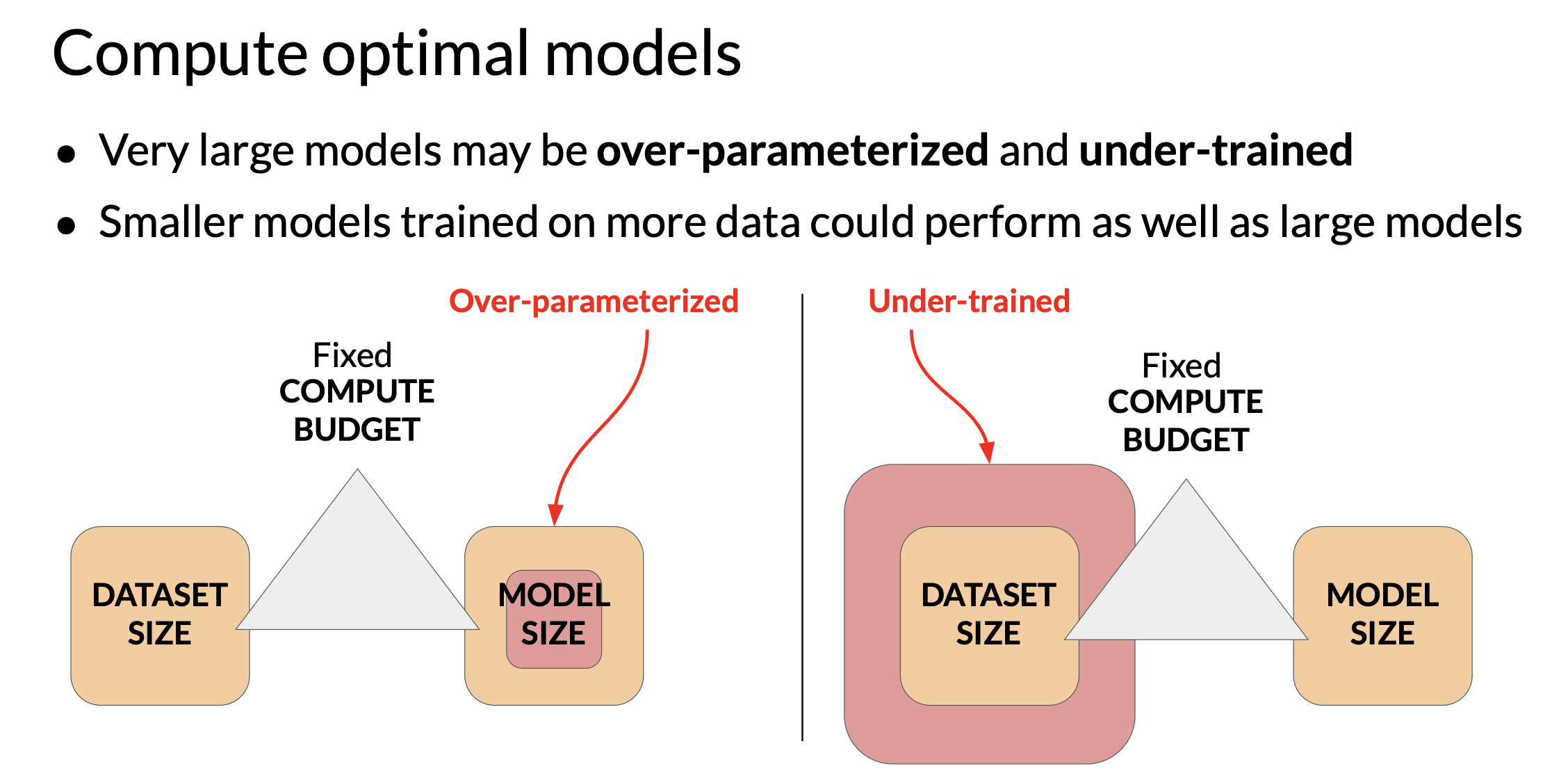
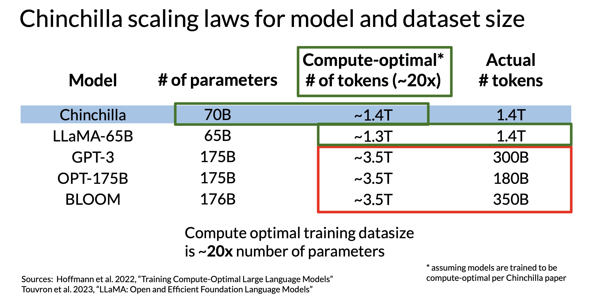
The Chinchilla scaling law shows that, for a fixed compute budget, language model performance is optimized by using more training data and a smaller model size (Hoffmann et al., 2022). Undertraining is the bottleneck - large models like GPT-3 were not trained on enough tokens to fully benefit from their size.
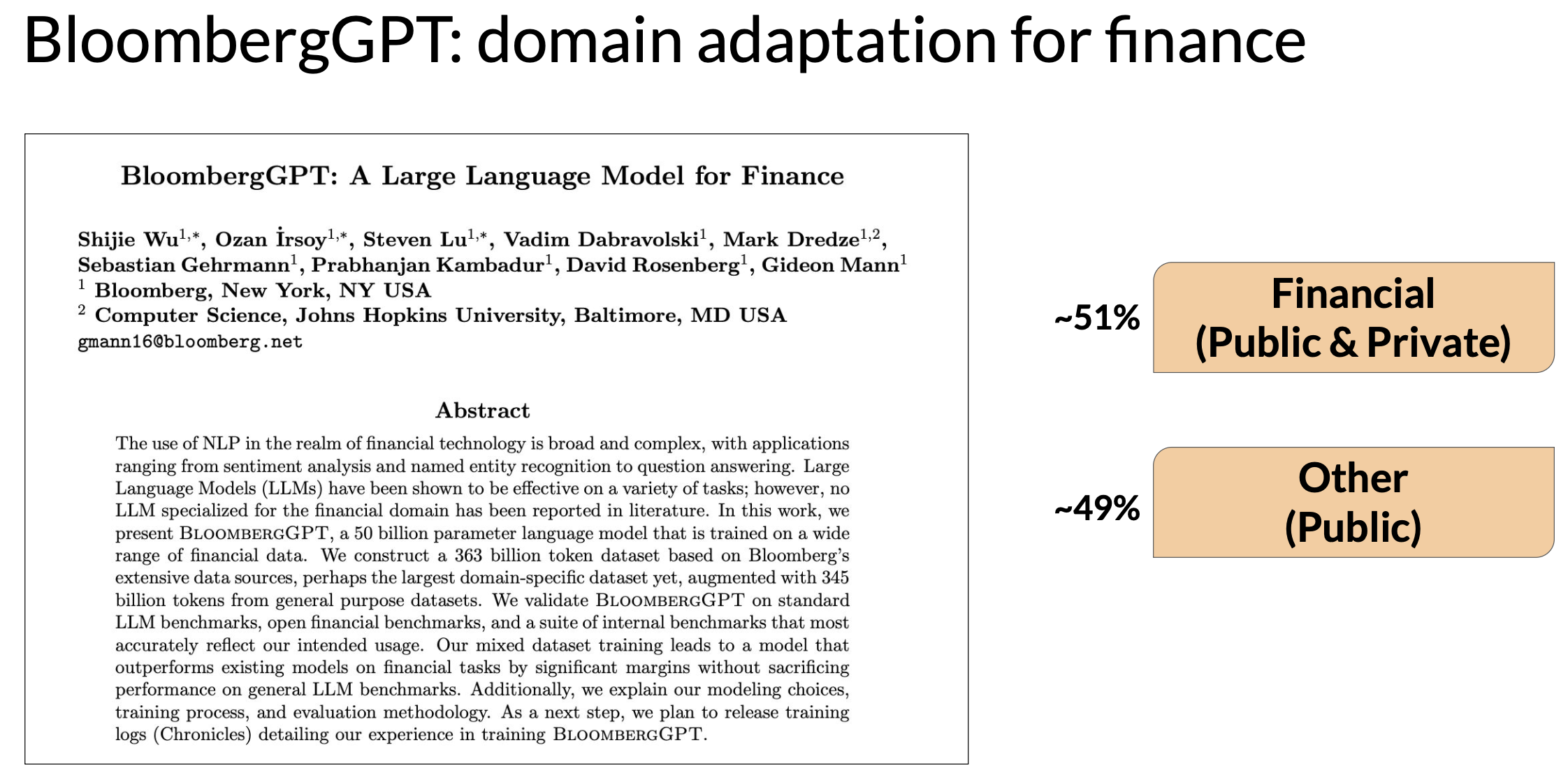
Domain adaptation
Example: BloombergGPT
References
- Generative AI on AWS: Building Context-Aware, Multimodal Reasoning Applications
- Deep dive into all phases of the generative AI Lifecycle
- BLOOM: BigScience 176B Model
- BLOOM is an open-source LLM with 176B parameters trained in an open and transparent way. In this paper, the authors present a detailed discussion of the dataset and process used to train the model. You can also see a high-level overview of the model here
- Vector Space Models
- Series of lessons from DeepLearning.AI’s Natural Language Processing specialization discussing the basics of vector space models and their use in language modeling.
- Scaling Laws for Neural Language Models
- Pre-training and scaling laws
- What Language Model Architecture and Pretraining Objective Work Best for Zero-Shot Generalization? Model architectures and pre-training objectives. The paper examines modeling choices in large pre-trained language models and identifies the optimal approach for zero-shot generalization.
- HuggingFace Tasks and Model Hub
- Collection of resources to tackle varying machine learning tasks using the HuggingFace library.
- LLaMA: Open and Efficient Foundation Language Models
- Article from Meta AI proposing Efficient LLMs (their model with 13B parameters outperform GPT3 with 175B parameters on most benchmarks)
- Language Models are Few-Shot Learners
- Scaling laws and compute-optimal models. This paper investigates the potential of few-shot learning in Large Language Models.
- Training Compute-Optimal Large Language Models
- Study from DeepMind to evaluate the optimal model size and number of tokens for training LLMs. Also known as “Chinchilla Paper”.
- BloombergGPT: A Large Language Model for Finance
- LLM trained specifically for the finance domain, a good example that tried to follow chinchilla laws.